NLP Series Part 1, Shapley and Interpretability is a must!
Disclaimer, for the sake of keeping these posts relatively short, I will not be conducting robust cross-validation, or using more advanced NLP techniques. This is purely to show a simple NLP multi-class classification task, and how we can interpret the results.
High Level Idea
Trying to convince your stakeholder that your model is a black box of magic that they can simply trust is, understandably, a hard sell. Shapley values are an absolute must and in my professional experience have been responsible for major buy in to a modeling effort.
Were going to do multi-class text classification, with 4 classes, show how to do summary plots, interpret an example for each of the 4 categories, and then show how an ambiguous sample is interpreted by all 4 classes.
To run this code you should use the requirements.txt as the versions of some packages are extremely important, and copy the model folder with the torch dense neural net implementation
Dataset: https://www.kaggle.com/datasets/tunguz/200000-jeopardy-questions
Code to run this yourself: https://github.com/AscherFriedman/AscherFriedman.github.io/tree/master/NLP_P1_Code
Includes modules that are in other directories and imports of packages
#Lets grab a csv containing historical information from the show jeapordy. Each Question belongs to a Category.
df = pd.read_csv('JEOPARDY_CSV.csv')
#Some of the columns come with odd names so lets strip white spaces before and after
df.rename(columns = {x:x.lstrip().rstrip() for x in df.columns}, inplace=True)
df = df[['Question','Category']]
df.Category.value_counts().head(10)
BEFORE & AFTER             547
SCIENCE                    519
LITERATURE                 496
AMERICAN HISTORY           418
POTPOURRI                  401
WORLD HISTORY              377
WORD ORIGINS               371
COLLEGES & UNIVERSITIES    351
HISTORY                    349
SPORTS                     342
Name: Category, dtype: int64
As we can see there are many many categories and they are all relatively small.
Lets create 4 categories by combining others: History, Literature, Art, and Geography
#rename_cols =
df.rename(columns = {x:x.lstrip().rstrip() for x in df.columns}, inplace=True) #EDA found spaces before and after column names
#Lets make some categories with 1500 observations each
df.Category.replace({'WORLD HISTORY':'HISTORY','AMERICAN HISTORY':'HISTORY','U.S. HISTORY':'HISTORY','THE CIVIL WAR':'HISTORY'},inplace=True)
df.Category.replace({'U.S. GEOGRAPHY':'GEOGRAPHY','WORLD GEOGRAPHY':'GEOGRAPHY',
                    'BODIES OF WATER':'GEOGRAPHY','ISLANDS':'GEOGRAPHY'},inplace=True)
df.Category.replace({'BOOKS & AUTHORS':'LITERATURE','SHAKESPEARE':'LITERATURE','FICTIONAL CHARACTERS':'LITERATURE','AMERICAN LITERATURE':'LITERATURE'},inplace=True)
df.Category.replace({'U.S. CITIES':'CITY_COUNTRY','STATE CAPITALS':'CITY_COUNTRY','WORLD CAPITALS':'CITY_COUNTRY'},inplace=True)
df.Category.replace({'ART & ARTISTS':'ART','BALLET':'ART','OPERA':'ART','MUSIC':'ART',
                    'CLASSICAL MUSIC':'ART'},inplace=True)
df = df[df.Category.isin(['HISTORY', 'LITERATURE', 'ART', 'GEOGRAPHY'])]
df.Category.value_counts()
HISTORY       1600
LITERATURE    1559
ART           1542
GEOGRAPHY     1507
Name: Category, dtype: int64
Lemmatizing and Speed
For a larger dataset I would suggest using the package pandarallel or using multiprocessing with an entire column at once as lemmatizing is known to be a slow process on large datasets. Mostly because it involves repeatedly using lookup tables for every word. Given this dataset is under 10,000 rows, lemmatizing is still quite fast.
stop_words = set(stopwords.words('english'))
wnl = WordNetLemmatizer()
# Two functions to do some basic cleaning, stripping odd characters and numbers, leaving alpha numeric.
def basic_clean(text):
    "Strips all non-alpha numeric text"
    # Regex pattern for only alphanumeric, hyphenated text
    return(re.sub(r'[^a-zA-Z -]', '', text))

def pre_processing(text):
    '''
    Tokenizes, Lemmatizes, Lower Cases, Removes Stopwords
    Joins back to Sentance'''
    lemma_list = ' '.join([wnl.lemmatize(x.lower()) for x in word_tokenize(text) if x.lower() not in stop_words])
    return lemma_list

df['clean'] = df['Question'].apply(basic_clean).apply(pre_processing)
Split Data
In another tutorial i’ll show how to better analyse results from a multi-class classification
#Label encoder for the the response variable
#Lets make the train and valid each 15% of the dataset
le = LabelEncoder().fit(df['Category'])
df['encoded'] = le.transform(df['Category'])
X_train, X_test, y_train, y_test = train_test_split(df['clean'], df['encoded'], test_size=.2, random_state=42,stratify=df['encoded'])
Very basic NLP algorithm
Convert to a tfidf matrix with 100 features, feed it into a 128,64,32 dense neural net with 4 classes using torch Then
#Vectorize to a tf-idf matrix max_features = 300 X_test_original = X_test.copy() #We save this tfidf matrix for the intepretation portion of this analysis tfidf = TfidfVectorizer(max_features=max_features) X_train = tfidf.fit_transform(X_train) X_test = tfidf.transform(X_test) feature_names = tfidf.get_feature_names_out ()
X_train = torch.tensor(X_train.todense()).to(device).float()
X_test = torch.tensor(X_test.todense()).to(device).float()

y_train = torch.tensor(y_train.values).to(device).float()
y_test = torch.tensor(y_test.values).to(device).float()
train_dataset = TFIDFDataset(X_train,y_train)
test_dataset = TFIDFDataset(X_test,y_test)

train_loader = DataLoader(dataset = train_dataset, batch_size = 32)
test_loader = DataLoader(dataset = test_dataset, batch_size = 16)
dataiter = iter(train_loader)
train_feat_ex, train_label_ex = dataiter.next()
model = dense_model(hidden_layers= [128,64,43], num_features = max_features, num_classes = len(le.classes_), p_drop=.15)
Again, this is a fairly small dataset and a non-robust cross validation procedure so these results are to be taken with a grain of salt, the point here is to highlight interpretation techniques, not performance
model, stats = train_nn(model, train_loader, test_loader, NUM_EPOCHS = 50, LR = .0001, LR_patience=5, early_stopping_callback= EarlyStoppingCallback())
  2%|█▋                                                                                 | 1/50 [00:00<00:43,  1.11it/s]

EPOCH 001: Loss: [Train: 1.36238 | test 1.24256 ] Accuracy: [Train: 31.964 | test 49.038] LR: 0.0001


  4%|███▎                                                                               | 2/50 [00:01<00:45,  1.05it/s]

EPOCH 002: Loss: [Train: 1.19640 | test 1.09368 ] Accuracy: [Train: 49.546 | test 64.103] LR: 0.0001


  6%|████▉                                                                              | 3/50 [00:02<00:43,  1.07it/s]

EPOCH 003: Loss: [Train: 1.04410 | test 0.94591 ] Accuracy: [Train: 61.679 | test 71.554] LR: 0.0001


  8%|██████▋                                                                            | 4/50 [00:03<00:43,  1.06it/s]

EPOCH 004: Loss: [Train: 0.92014 | test 0.84137 ] Accuracy: [Train: 68.717 | test 75.689] LR: 0.0001


 10%|████████▎                                                                          | 5/50 [00:04<00:41,  1.08it/s]

Message from callback (Early Stopping) counter: 1/5
no
EPOCH 005: Loss: [Train: 0.81978 | test 0.75311 ] Accuracy: [Train: 72.583 | test 77.420] LR: 0.0001


 12%|█████████▉                                                                         | 6/50 [00:05<00:40,  1.09it/s]

EPOCH 006: Loss: [Train: 0.72940 | test 0.68310 ] Accuracy: [Train: 75.935 | test 78.141] LR: 0.0001


 14%|███████████▌                                                                       | 7/50 [00:06<00:38,  1.11it/s]

Message from callback (Early Stopping) counter: 1/5
no
EPOCH 007: Loss: [Train: 0.66856 | test 0.63342 ] Accuracy: [Train: 77.958 | test 78.622] LR: 0.0001


 16%|█████████████▎                                                                     | 8/50 [00:07<00:37,  1.12it/s]

Message from callback (Early Stopping) counter: 2/5
no
EPOCH 008: Loss: [Train: 0.62259 | test 0.63164 ] Accuracy: [Train: 80.195 | test 78.990] LR: 1e-05


 18%|██████████████▉                                                                    | 9/50 [00:08<00:36,  1.12it/s]

Message from callback (Early Stopping) counter: 3/5
no
EPOCH 009: Loss: [Train: 0.61857 | test 0.62941 ] Accuracy: [Train: 80.442 | test 78.429] LR: 1e-05


 20%|████████████████▍                                                                 | 10/50 [00:09<00:36,  1.11it/s]

Message from callback (Early Stopping) counter: 4/5
no
EPOCH 010: Loss: [Train: 0.60936 | test 0.62494 ] Accuracy: [Train: 80.863 | test 79.151] LR: 1e-05


 20%|████████████████▍                                                                 | 10/50 [00:10<00:40,  1.00s/it]

Message from callback (Early Stopping) counter: 5/5
here
Training stopped -> Eearly Stopping Callback : test_loss: 0.6211988784563847
For the Shap package, deep explainer generally works fairly quick to nn.torch problems that arnt image classification
explainer = shap.DeepExplainer(model, shap.sample(X_test,25))
# Get the shap values from my test data
shap_values = explainer.shap_values(X_test)
%matplotlib inline
Functions to generate plots
Worth noting that the title option on shap plots is buggy, so we turn it off, add it manually matplotlib
def summary(feature):
    encoded = le.transform([feature])[0]
    shap.summary_plot(shap_values[encoded],X_test.cpu(), feature_names=feature_names, class_names=le.classes_,show=False)
    plt.title(feature,fontsize=16)
    plt.savefig(feature,bbox_inches='tight')
    plt.close()

def specific_example(feature,threshold,sample_num, save_fig = False):
    encoded = le.transform([feature])[0]
    sample_index = np.where(y_test.cpu().numpy()==encoded)[0][sample_num]
    shap_vals = shap_values[encoded][sample_index]
    use = shap_vals*[abs(shap_vals)>threshold][0]
    shap.bar_plot(use,feature_names=feature_names,max_display=(abs(use)>0).sum(),show=False)
    sentence  = df.loc[X_test_original.index[sample_index],'Question']
    plt.title(f'{feature} sample: "{sentence}"')
    if save_fig:
        plt.savefig(feature+'_barplot',bbox_inches='tight')
    plt.close()
Create Summary plot for all 4 classes
for feature in le.classes_[:]:
    summary(feature)
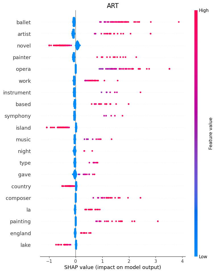
Note that in these shaply plots a word either exists or it doesnt, so blue just means no word, and red means words are in the sentance we are plotting.
ART
Here we can see that words such as “Ballet”, “Artist”, “Painter” and “Opera” tell the model that the question belongs to category ART.
If it sees “Island” or “Novel”, it is a good indication that it is not art.
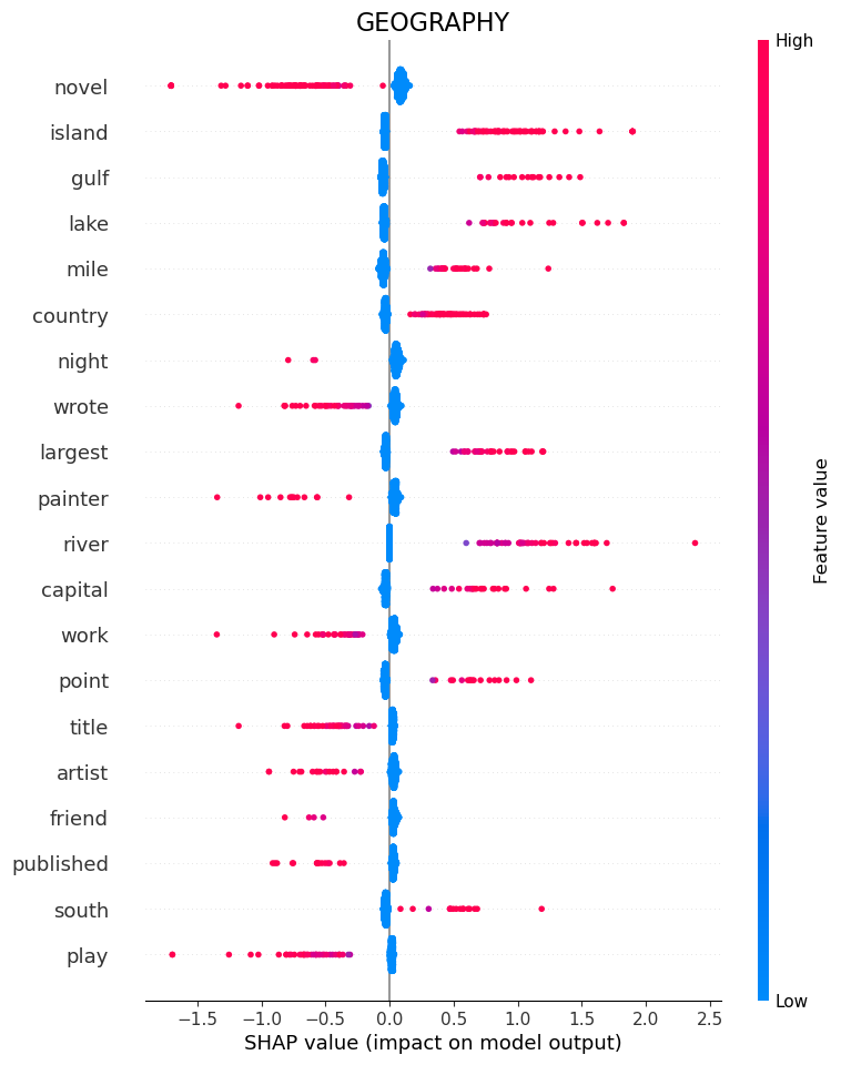
Geography
“Island”, “Gulf”, “Lake” and “Mile” tell the model that the question belongs to category Geography.
If it sees “Wrote” or again “Novel”, it is a good indication that it is not geography.
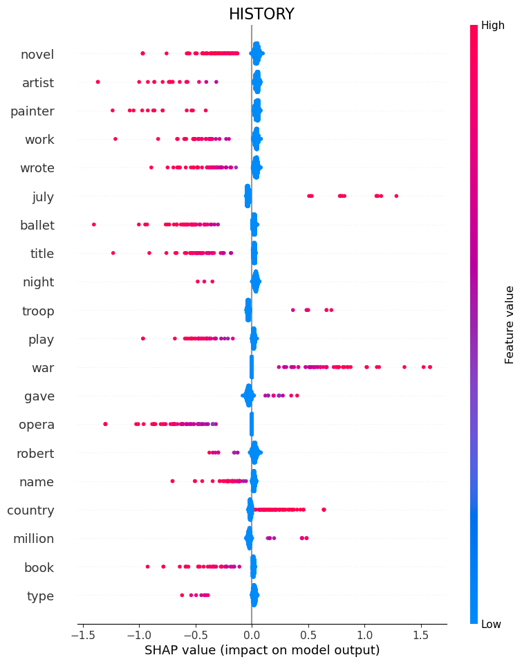
History
History is an interesting case because the model is primarily defined by which words are not present.
So if it sees “Novel” or “Artist” or “Wrote”, it knows its not history.
Some words are still positive Indicators, like “War”.
Literature
“Novel”, “Wrote”, “Published” and “Book” tell the model that the question belongs to category Literature.
If it sees “island” or “Country”, it is a good indication that it is not literature.
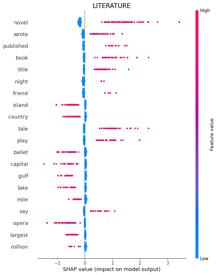
“Novel” ends up being important because theres a category that we combined into Literature called “Novels” so each question in that subcategory had the word Novel in it.
Picked some specific examples that are interesting to look at
specific_example('ART',.1,3, save_fig=True)
specific_example('HISTORY', .1, 1, save_fig=True)
specific_example('GEOGRAPHY', .1, 5, save_fig=True)
specific_example('LITERATURE', .1, 9, save_fig=True)
ART
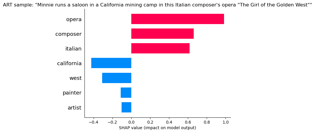 “Opera” and “Composer” indicate its ART, but “California” and “West” indicate its not art! Still we can see the positives are much larger than the negatives and the model still likely choses art.
Geography
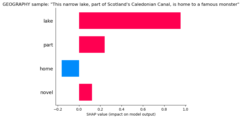 “Lake and “Part” tell the model its geography, but “Home” is a small hint it might not be (home probably belongs frequently to literature and history.
History
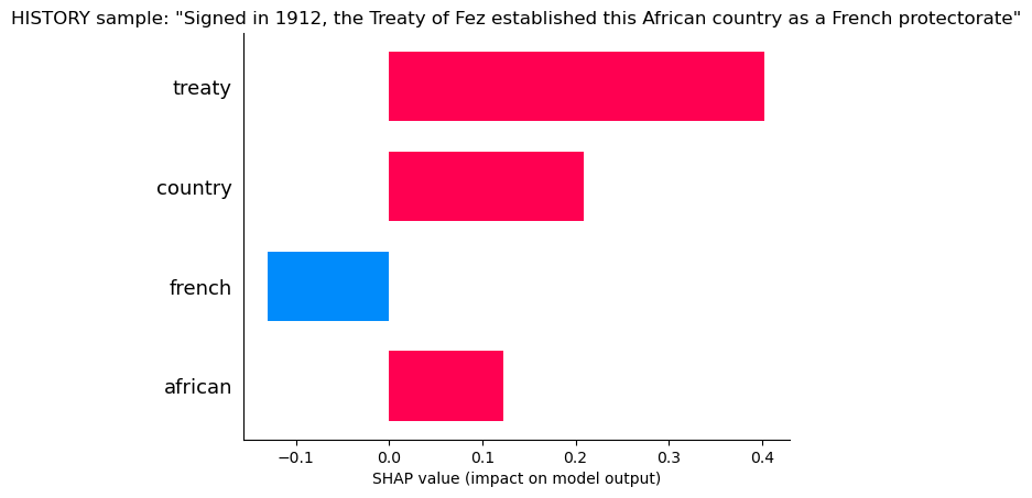 “Treaty” and “Country” tell the model it is likely History, but “French” says it may not be, probably because of many French Artists.
Literature
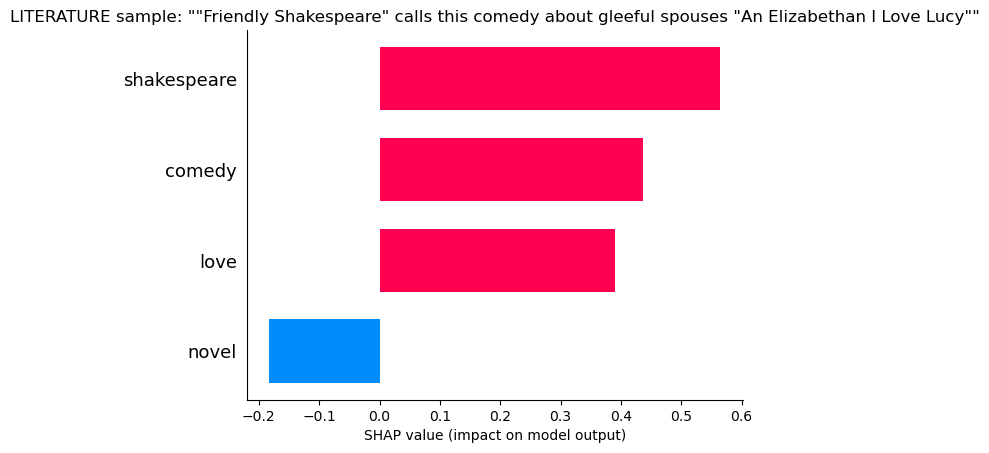 “Shakespear”, “Comedy”, “Love”, all hallmarks of literature, but so many literature questions contained the word “Novel” that the lack of this word makes the model uncertain
Lets Pick an interesting and very confliting case and see how the model evaluates the likelyhood of each category.
“Tradition says this country’s first emperor, Menelik 1, was the son of King Solomon and the Queen of Sheba” This is a history question.
for feature in le.classes_:
    encoded = le.transform(['HISTORY'])[0]
    sample_index = np.where(y_test.cpu().numpy() == encoded)[0][32]
    shap_vals = shap_values[le.transform([feature])[0]][sample_index]
    use = shap_vals*[abs(shap_vals) > .05][0]
    shap.bar_plot(use,feature_names = feature_names,max_display = (abs(use) > 0).sum(),show = False)
    sentence  = df.loc[X_test_original.index[sample_index],'Question']
    plt.title(f'{feature} sample: "{sentence}"')
    plt.savefig(feature+'_one_sample_mult_feat_',bbox_inches='tight')
    plt.show()
ART
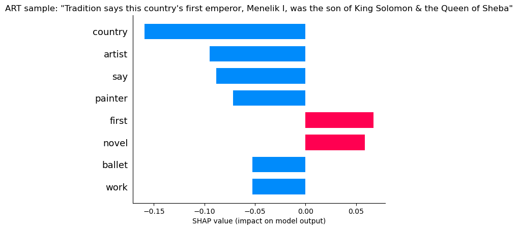 The presence of words like “Country” and “Say” and “First”, as well as the absence of words like “Artist” and “Painter” all indicate this is not ART.
Art is ruled out!
The presence of words like “Country” and “Say” and “First”, as well as the absence of words like “Artist” and “Painter” all indicate this is not ART.
Art is ruled out!
Geography
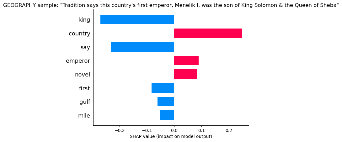 Geography sees words like country that give it some confidence, but “Say” and “King” are enough to know its not Geography.
Geography is ruled out!
Geography sees words like country that give it some confidence, but “Say” and “King” are enough to know its not Geography.
Geography is ruled out!
History
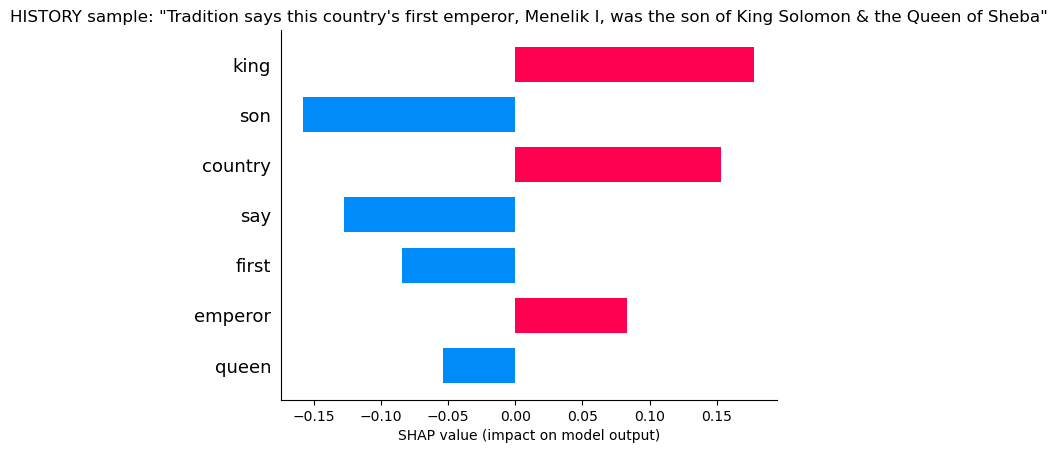 Here the model sees “King” and “Country” giving it confidence, but also “Say”, “First” and “Son” which makes it doubtful. Say usually belongs to literature, as does Son.
Literature
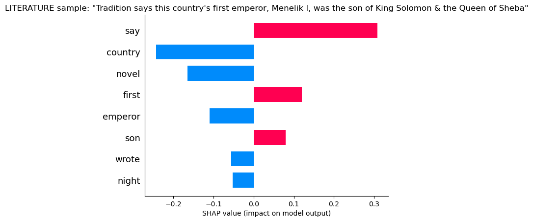 Here the model sees “Say”, “First” and “Son”, which are frequently found in literature, but it still has doubts given that it sees “Country” and “Emperor” and no “Novel”
print('True Label:',df.loc[X_test_original.index[sample_index]].Category)
probs = np.array(softmax(model(X_test[sample_index:sample_index+1]),dim=1).detach().cpu())[0]
print()
for category,prob in zip(le.classes_,probs):
    print(f'{round(prob*100,2)}% chance of being {category}')
print()
print('Modle Predicts: ', le.classes_[probs.argmax()])
True Label: HISTORY

14.71% chance of being ART
17.11% chance of being GEOGRAPHY
33.44% chance of being HISTORY
34.74% chance of being LITERATURE

Modle Predicts:  LITERATURE
The model is just barely wrong! With a little hyperparameter tuning, or simple tricks like adding in bi-grams, i’m sure it can figure it out!